

The first generation of wireless PC accessories to achieve widespread success (the ones that shipped with a dongle in the box) adopted 2.4GHz radios because these radios offered the optimal trade-off between power consumption, throughput, and range. Nordic Semiconductor's radios were a popular choice in these accessories and, as a result, many devices on the market today still use the legacy ShockBurst (SB) and Enhanced ShockBurst (ESB) packet formats that Nordic introduced starting in 2004. This isn't too surprising because proprietary radio packets are just as useful today as they were then; low-level access to the radio offers performance and flexibility that protocols such as Bluetooth Low Energy (BLE) cannot match. Not only are SB and ESB compatible with the same radio as BLE, contemporary Nordic devices allow the application to use them and BLE concurrently.
Here is an overview of the radio:
- GFSK modulation
- 2.4GHz ISM band
- 250kbps (legacy devices only), 1Mbps, or 2Mbps bitrates
- 1MHz (250kbps, 1Mbps) or 2Mhz (2Mbps) channel spacing
- 64 (legacy) or 100 selectable channel frequencies
- Up to 20dBm transmit power (typically not more than 4dBm)
Comprehensive documentation --including low-level details like CRC polynomials-- can be found in the data sheets of legacy Nordic devices.
The official User Guide provides a nice overview of the original star-network use case, some radio activity diagrams, and a taste of the API.
The Packet
The SB packet format looks like this:
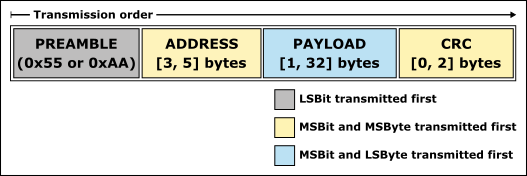
Although this format uses the radio very efficiently, it doesn't provide any extra features. For example, both sides of the link need to be configured to use the same payload length before transmitting anything because that is not described anywhere in the packet.
Enhance!
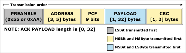
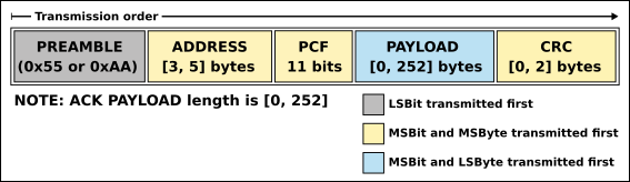
Changes were quickly made to the original SB packet format in order to allow the hardware to do some additional processing. The new format is referred to as Enhanced ShockBurst (ESB). ESB packets on legacy devices support payloads of up to 32 bytes:
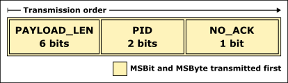
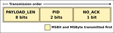
In addition to making the CRC field mandatory, a Packet Control Field (PCF) was introduced. Note that on legacy devices the PAYLOAD_LEN is fixed to 6 bits:
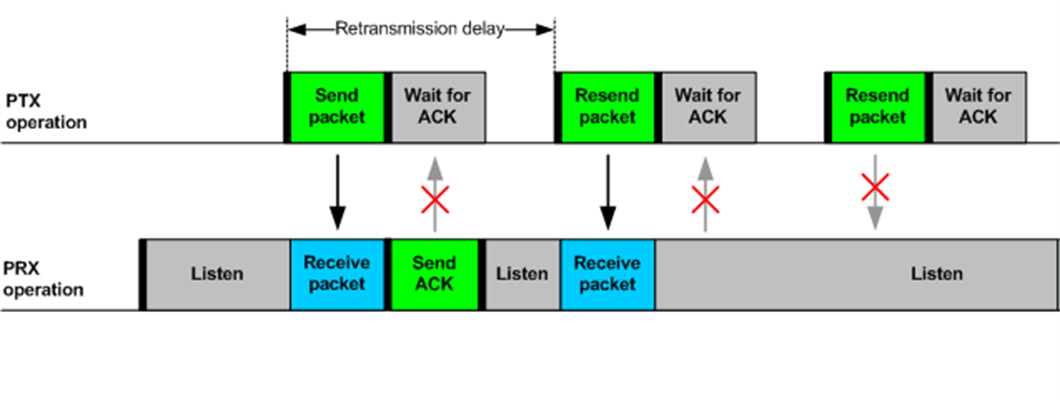
The new payload length field, packet ID, and an acknowledge bit mean that payload lengths can be dynamic, packets can be acknowledged by the receiver, and unacknowledged packets can be automatically retried. If an acknowledgement is required then it can contain a payload in order to facilitate bidirectional communication. Note that acknowledgement payloads must be preloaded; it is not possible for a transmitter to send a command and receive a direct response to that command in the acknowledgement. Instead, the response would have to be preloaded so it could be sent as the acknowledgement for the next command that is received. Preloaded acknowledgement payloads are required in order to guarantee that acknowledgement timing is deterministic.
Contemporary devices can use an updated ESB packet format as long as backwards compatibility with legacy devices is not required. The new format allows for empty payloads --which is useful when sending polling packets-- along with an expanded payload length of up to 252 bytes. The CRC bytes were also made optional (though using 2 bytes is recommended):
Note that the PAYLOAD_LEN in the updated PCF is increased to 8 bits when larger payloads are enabled:
Timing
The amount of on-air time that is required to send a particular packet is primarily determined by the packet's length and the bitrate of the physical layer. Additionally, radios have a ramp-up time that is required whenever the radio switches mode from disabled to RX or TX. There is also usually a short delay while receiving a packet or disabling the radio. The radio can't transmit or receive during these periods so it's practical to include them when calculating radio time budgets. The nominal ramp-up time for legacy SB devices is 130us. nRF52 devices can shorten this ramp-up to 40us if backwards compatibility is not required.
Working with ESB
Prior to the nRF51 series the radio hardware handled most of the ESB features, including generating acknowledgements, without CPU intervention. However, the additional processing power in contemporary devices now allows for an ideal split between hardware and software -- the radio takes care of low-level activity and keeps timing deterministic while everything else is handled in software for maximum flexibility. This allows for novel use cases like adding a small amount of ESB to a BLE device for sub-microsecond time synchronization. At the other end of the spectrum are products that implement bespoke proprietary networks to achieve aggressive optimization for latency, throughput, or reliability. The application gets to decide:
- When to send or receive packets
- Address and frequency for each packet
- TX output power for each packet exchange
- Optional ACK packet back from peer (with optional payload)
- Payload lengths
- Discard or retry dropped packets
This is accomplished by integrating the ESB source code from the SDK directly into the application and modifying the reference ESB implementation as necessary to support requirements. Note that there is no implementation for the original ShockBurst packet format even though it's still supported by the hardware. Additionally, hardware support for the 250kbps bitrate was discontinued starting with the nRF52 series.
Consider an example use case that's difficult with BLE; there is one transmitter that needs to broadcast 50 bytes of common data to ten peer nodes and then reach out to each of the peers individually to send 5 more bytes and receive another 30 bytes. All of the nodes in the network will use the same address for the broadcast packet and the receiver nodes will then use the time that the broadcast packet is received to determine when to listen for their individual polling packets. Assuming that the popular 2mbps bitrate is used this simple Python script can calculate the radio budget for nRF52/nRF53 devices:
>>> from esb_timing import *
>>> pkt_len_tx_2mbps_us(50)
281.5
>>> pkt_len_tx_w_ack_2mbps_us(5, 30)
305.0
Some napkin math might look like this:
- TX sends 50 bytes with no ACK requested (282us)
- TX sends 5 bytes to RX_1 and receives 30 bytes in the ACK packet (305us)
- ...
- TX sends 5 bytes to RX_10 and receives 30 bytes in the ACK packet (305us)
This means that the initial broadcast plus 10x polling exchanges with peers (0.282ms + 10 * 0.305ms) only reqiures ~3.4ms of radio time. Of course this is a lower bound but even with some additional slack to account for e.g. sensor data acquisition this network with 11 total nodes could potentially operate at close to 200Hz.
Conclusion
The ESB protocol allows low-level access to the radio and should be considered any time optimization or flexibility is required between two or more Nordic devices. Furthermore, the Multiprotocol Service Layer Timeslot makes it possible to leverage the strengths of ESB concurrently with standard protocols like BLE.

Top Comments
-

Daniel Veilleux
-
Cancel
-
Vote Up
+1
Vote Down
-
-
Sign in to reply
-
More
-
Cancel
Comment-

Daniel Veilleux
-
Cancel
-
Vote Up
+1
Vote Down
-
-
Sign in to reply
-
More
-
Cancel
Children