

This is an updated field test of the one we did in 2019 at the same location. During this updated field test, we also captured more parameters for both LTE-M and NB-IoT devices and, we captured power measurements of the cellular devices on each kilometer from the base station.
Table of Contents
Introduction
There are many sources online that try to characterize LTE-M (Cat-M1) and NB-IoT (Cat-NB1) technologies. Unfortunately, many of these characterizations list ideal numbers which are not applicable in the real world. In the context of power consumption, we also need to consider the network configurations which have a major impact on the overall power consumption of the User Equipment (UE). That is the reason we initiated this field test using Nordic Semiconductor’s nRF9160 System in Package (SiP) as the UE to explore these areas.
In this field test we have captured several data parameters, captured the power consumption of the device, and used the Nordic specific connection evaluation feature to evaluate the network link before sending Uplink (UL) data using UDP (User Datagram Protocol). This was captured both using LTE-M and NB-IoT technologies with an interval of 1 km away from the base station (technical term “eNB”). The measurements were taken while the devices were static and from a cold start at each location.
We will begin this field test blog with some background information around the differences between LTE-M and NB-IoT technology and the different modes a cellular modem can be in. The next section will go through the execution of the field test, what tools were used and how we performed the measurements. After that, we will jump into the results section showing what we captured during our test. The section after that will be discussing the results we found and at the end we will have a conclusion section for this field test. We also have an LTE abbreviations section at the bottom for you to look up any abbreviations that are used in this blog.
Background
There are a couple of relevant differences between LTE-M and NB-IoT that are worth mentioning before continuing. Let us look at the overview table comparing LTE-M and NB-IoT taken from us “What is Cellular IoT?” page.
Table 1 Difference between LTE-M and NB-IoT
|
|
LTE-M |
NB-IoT |
|
Also known as |
“eMTC”,”LTE Cat-M1” |
“LTE Cat-NB1” (3GPP rel 13) - "LTE Cat-NB2" (3GPP rel 14) |
|
Bandwidth |
1.4 MHz |
200 kHz |
|
Max Throughput |
300/375 kbps |
30/60 kbps (NB1) - |
|
Range |
Up to 4x |
Up to 7x |
|
Mobility/cell re-selection |
Yes |
Limited |
|
Frequency deployment |
LTE In-band |
LTE In-band, guard band and GSM (Global System for Mobile) re-purposing |
|
Deployment density |
Up to 50,000 per cell |
Up to 50,000 per cell |
|
Module size |
Suitable for wearables |
Suitable for wearables |
|
Power consumption |
Up to 10 years of battery lifetime |
Up to 10 years of battery lifetime |
Firstly, the on-air bandwidth is different. LTE-M has 1.4 MHz, while NB-IoT has 200 kHz. The bigger bandwidth of LTE-M results in higher throughput, while the smaller bandwidth of NB-IoT should result in better signal quality and longer range. This means that under the same network conditions and when sending the same amount of data, LTE-M will be the recommended technology to use for low power operations since it requires less time to have the radio ON because of the higher throughput compared to NB-IoT.
Let us now look at the different modes an LTE-M/NB-IoT modem can be in.
There are three main modes:
- RRC (Radio Resource Control) Connected mode
In this mode, the radio is active, and the modem must stay in synchronization with the network, which requires the high accuracy timers in the UE to be enabled. This mode causes the most power consumption and for low power devices you want to be in this mode as rarely as you can depending on your application’s needs.
- RRC Idle mode
In this mode, you do not need to stay in synchronization with the network. The transceiver is turned OFF and you utilize the eDRX intervals to sleep in between the paging windows where you turn ON the receiver to check if there is some data from the network that you can receive. If the network has some data for the UE, the modem will go back to RRC connected mode. The UE can request the eDRX interval, but the network decides if it will allow you this interval or not. What we commonly see is that the networks approve extending this interval more often than shortening it
- Power Saving mode (PSM)
In this mode, the radio is off all together and the UE is unreachable from the network side. The UE is still registered to the network so when it wakes up and goes to RRC Connected mode it does not need to search for a network and register again, which the modem must do if you turn it off instead of using PSM. The UE can stay in PSM for intervals of ~6 minutes, up to several weeks depending on the network. NOTE: Some networks do not grant roaming devices PSM or eDRX features, this is specified by the agreements between the roaming SIM card and the local network carrier.
What should be noted is that an nRF9160 device in PSM mode can wake itself up when it wants to and go to RRC Connected mode if it needs to send data, e.g. an alarm.
PSM floor current is 2,7µA for the nRF9160 SiP.
The application can use a combination of modes, depending on what you need in your application. A great rule of thumb for low-power devices is to send a lot of data as infrequently as possible. In that way, you avoid going in and out of RRC connected mode often and can for instance benefit from being in PSM for most of the time to minimize power consumption.
An application will typically use one of the following configurations:
- RRC connected, RRC Idle and PSM
- RRC connected and RRC Idle (Figure 1)
- RRC connected and PSM (Figure 2)
Let us first look at the RRC Connected and RRC Idle modes with the waveform captured from the Online Power profiler which is used to estimate power consumption on the nRF9160 SiP.
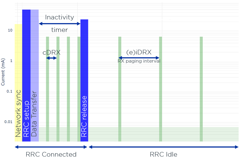
Figure 1 RRC Connected and RRC Idle mode
Figure 1 shows how the nRF9160 SiP connects to a network, sends some UDP data, and then goes into RRC Idle mode which listens for incoming messages from the network in intervals that are referred to as iDRX intervals. This is the interval that is referred to when you read typical marketing material around eDRX, but the definition of eDRX is “intervals above 5.12s” so it can also be used in the context of cDRX but it rarely is. The cDRX interval is “connected-DRX” in the RRC Connected mode and is configured by the network and cannot be changed by the UE. That is why we will address eDRX as iDRX in this blog to be precise and to avoid confusion. As you can see in Figure 1 you have an interval in RRC Connected mode which is referred to as cDRX. This interval is set by the network and cannot be requested to be changed from the UE. In contrast we have the iDRX interval where the UE can request the network for another iDRX interval using the AT command “+CEDRXS” or through our LTE Link Controller library in nRF Connect SDK. The cDRX intervals are usually much shorter than the typical iDRX intervals. cDRX can be between the intervals 0.01s to 10.24s, while iDRX intervals can be requested to be between 0.16s up to ~44min. This means that when using RRC Connected mode and RRC Idle mode, iDRX intervals potentially have a more significant impact on the overall power consumption than cDRX.
Another important parameter in RRC Connected mode is the “inactivity timer” more precisely known as the “RRC inactivity timer.” Like cDRX, this timer is also configured by the network. The purpose of the RRC inactivity timer is for the network to keep the UE connected in case there is any additional data coming since the network does not know when the last packet is sent. However, this additional time of staying in RRC Connected mode can be detrimental to the power budget if the network has configured this timer to be too long, since you must wait for this timer each time you want to go out of RRC Connected Mode. Some networks could have this RRC inactivity timer set at 4 seconds while others can have it set to 18 seconds, and this can potentially reduce your battery life in half.
Try this yourself to experiment with network configurations and parameters in the Online Power Profiler.
Now let us look at the RRC Connected Mode and PSM combination which is what is used in our field test.
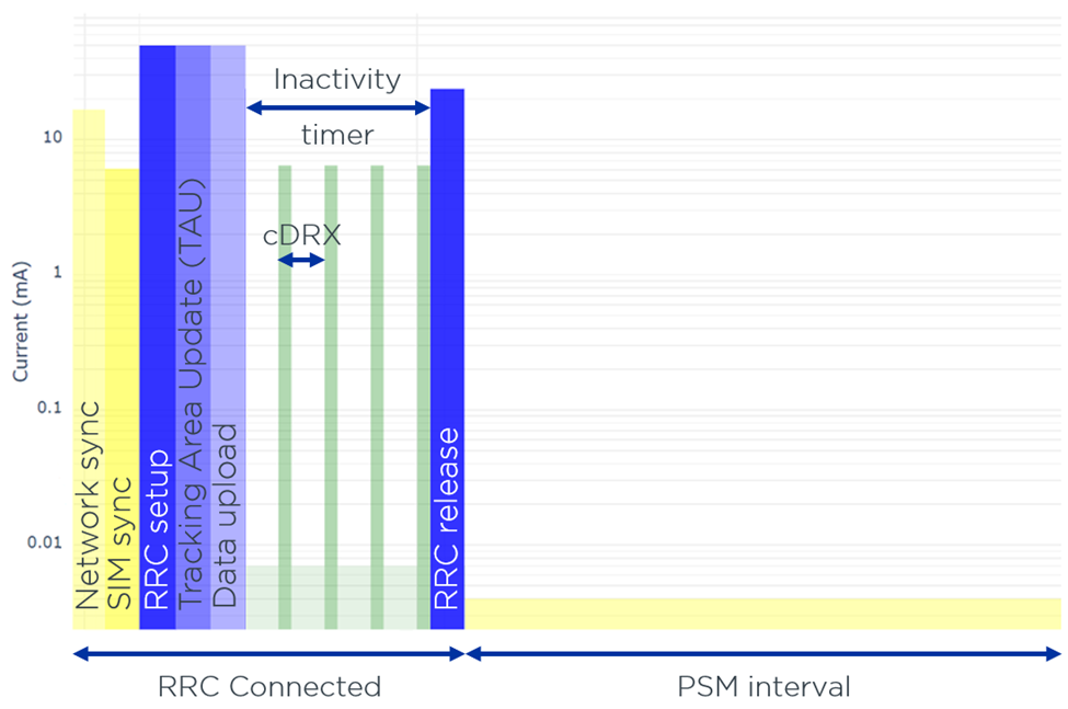
Figure 2 RRC Connected mode and PSM
Figure 2 shows how the nRF9160 SiP wakes up from PSM and re-connects to the network, sends some UDP data and then goes back into Power Saving Mode. In PSM, the UE is still registered to the network but can shut down the modem for an approved interval by the network (this is handled automatically by the modem). That means that while in PSM the UE is unreachable by the network but can wake up at any time to send data. The PSM interval (also known as Periodic TAU or T3412 timer) can in theory be between 10 min up to 413 days (about 1 year 1 and a half months) and can be requested by the AT command “+CPSMS” or the LTE Link Controller library. This interval specifies how often the UE is required to wake up from PSM to do a Tracking Area Update (TAU). Explained simply, this is just for the network to know where the UE is located, i.e. the tracking area. If you wake up from PSM to transfer data (or any other activity that requires the UE to attach to the network) it will always perform the TAU procedure, and hence the periodic TAU timer is reset.
Execution
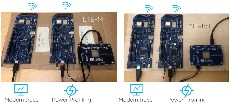
Figure 3 Test setup for the field test using nRF9160 DK and PPK2
We used the standard (v1.0.1) together with SIM cards from the Norwegian mobile operator Telenor. We also used the to measure the power consumption of two selected nRF9160 DKs as seen in Figure 3. The modem firmware we used during our testing was modem firmware v1.3.1. We used 4 different nRF9160 DKs running 4 different versions of the UDP sample in nRF Connect SDK, with slightly different configurations.
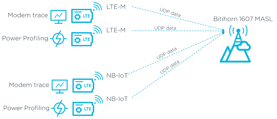
Figure 4 The full test setup used in this field test
The following was our setup, also shown in Figure 4:
- 1 x nRF9160 DK running UDP sample with modem trace enabled and LTE-M enabled
- 1 x nRF9160 DK running UDP sample with modem trace disabled and LTE-M enabled with power consumption measurements
- 1 x nRF9160 DK running UDP sample with modem trace enabled and NB-IoT enabled
- 1 x nRF9160 DK running UDP sample with modem trace disabled and NB-IoT enabled with power consumption measurements
We measured power consumption on the nRF9160 SiP DKs that did not have modem trace enabled since this feature draws extra current and would affect the power measurements.
NOTE: This distinction is particularly important in this field test since we cannot 100% correlate the modem trace data with the power measurement data using the same network technology because the data was captured on two separate DK. However, it should still give us a good overall picture of what affects the power consumption with regards to the traces we took from the other DKs.
It is based on the UDP sample from our nRF Connect SDK, but we increased the “CONFIG_UDP_DATA_UPLOAD_SIZE_BYTES” to 300 bytes and enabled modem trace on two of the samples, one where the “CONFIG_LTE_NETWORK_MODE_LTE_M” is enabled and one with “CONFIG_LTE_NETWORK_MODE_NBIOT” enabled. We also included several AT commands to read out different parameters that we thought would be interesting to track. These commands were +CGMR, %XMONITOR, +CESQ, %XSNRSQ, %XTEMP, +CEINFO and %CONEVAL.
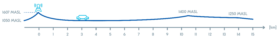
Figure 5 Showcasing our drive away from the eNB
We began our measurements 3 km from the base station (eNB) that is at the top of the mountain Bitihorn. We measured power consumption for the two DKs while connecting to the network and capture the modem traces on the other two DKs from bootup until they went in to PSM. Then we drove north 1 km from our first test point at 3 km and repeated the same process of data and power measurements from bootup until the devices went to PSM. This process continued until we lost connection on all our devices. All measurements were taken while the devices were static.
Results
LTE-M technology results
Let us begin with the data we captured on the DKs connected to the LTE-M network.
First, we will look at the network-specific configurations (Table 2) we got from the base station (eNB) at the top of mountain. These values can be read out from the waveform captured using the Power Profiler Kit II. If you want to do this yourself on your network, you can follow this YouTube tutorial. The increased values we see in red for NB-IoT in Table 2 should have a negative impact on overall power consumption and what we see in green should decrease the power consumption. You can use the Online Power Profiler and check this yourself.
Table 2 Network specific configurations for LTE-M and NB-IoT on the eNB
|
Description |
LTE-M |
NB-IoT |
Difference in NB-IoT |
|
RRC inactivity timer (ms) |
11000 |
18000 |
7000 |
|
cDRX Interval (ms) |
320 |
2048 |
1728 |
|
cDRX ON duration (ms) |
40 |
60 |
20 |
|
cDRX inactivity timer (ms) |
100 |
50 |
-50 |
Below, we can see Table 3 which displays a lot of different parameters captured from the AT commands that we sent and read out using modem traces (can also be read out from the serial output log of the application). You can click on the description titles to check which specific AT command was used for the different parameters. Blue numbers stay consistent for each kilometer away from the base station. We could not connect to the LTE-M network after 12 km (about 7.46 mi).
Table 3 Data captured from the modem trace on the LTE-M network
|
Description |
3 km |
4 km |
5 km |
6 km |
7 km |
8 km |
9 km |
10 km |
11 km |
12 km |
|
23 |
8 |
15 |
15 |
15 |
15 |
15 |
16 |
23 |
23 |
|
|
-101 |
-82 |
-75 |
-95 |
-94 |
-94 |
-89 |
-92 |
-102 |
-105 |
|
|
7 -Normal |
8 - Good |
8 - Good |
7 -Normal |
7 -Normal |
7 -Normal |
7 -Normal |
7 -Normal |
7 -Normal |
7 -Normal |
|
|
Time to get connected (sec) |
3,4 |
4,5 |
3,5 |
4,8 |
4,2 |
4,2 |
3,8 |
4 |
4,2 |
3,5 |
|
5 |
16 |
19 |
12 |
12 |
11 |
16 |
12 |
7 |
4 |
|
|
1 |
1 |
1 |
1 |
1 |
1 |
1 |
1 |
1 |
1 |
|
|
8 |
8 |
8 |
8 |
8 |
8 |
8 |
8 |
8 |
8 |
|
|
1 |
1 |
1 |
1 |
1 |
1 |
1 |
1 |
1 |
1 |
|
|
1 |
1 |
1 |
1 |
1 |
1 |
1 |
1 |
4 |
4 |
|
|
5 |
15 |
18 |
13 |
10 |
11 |
15 |
12 |
7 |
4 |
In Figure 6, we highlight the correlation between the TX Output Power and RSRP for each kilometer from the base station as well the energy estimates seen from Table 3.
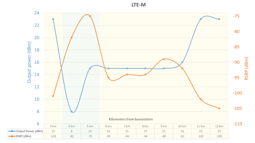
Figure 6 Correlation of Output power and RSRP on LTE-M
Figure 6 shows the output power on the left axis and the RSRP on the right axis. The bottom table shows the kilometers from the base station (eNB) with the actual measurements. Typically, the higher the RSRP, the better the signal quality, e.g. -75 dBm is better signal quality than -105 dBm. The background colors represent the energy estimates from Table 3, so we can see at 4 km it is estimated to be “good conditions”.
Let us now look at how the power consumption in Figure 7 is affected by increasing the distance between the eNB and the UE.
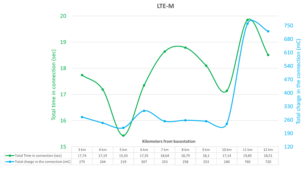
Figure 7 Total time and total charge captured during the connection in LTE-M
From Figure 7, we can see the correlation between the total time in the connection and the total charge of the connection, which is measured from the boot up of the nRF9160 SiP until it goes to Power Saving Mode. You can use these numbers to calculate what the average total power consumption is and use that to calculate battery lifetime. This can give you an overview of how the power consumption of a device is affected by distance (or obstructions) from the eNB.
NB-IoT technology results
Following we see Table 4 that includes all the different parameters captured from the AT commands we sent for the UE using the NB-IoT network. You can click on the description titles to check which specific AT command was used for the different parameters. Blue numbers stay consistent for each kilometer away from the base station. We showcase the results from 3 -12 km (about 7.46 mi), since after 12 km the NB-IoT device connected to a different eNB.
Table 4 Data captured from the modem trace on NB-IoT
|
Description |
3 km |
4 km |
5 km |
6 km |
7 km |
8 km |
9 km |
10 km |
11 km |
12 km |
|
21 |
4 |
3 |
2 |
8 |
4 |
10 |
14 |
21 |
22 |
|
|
-90 |
-66 |
-66 |
-65 |
-70 |
-73 |
-74 |
-76 |
-88 |
-90 |
|
|
7 -Normal |
8 - Good |
7 - Normal |
8 - Good |
7 - Normal |
8 - Good |
7 - Normal |
7 - Normal |
7 - Normal |
6 - Poor |
|
|
Time to get connected (sec) |
19 |
22,6 |
19,2 |
26,2 |
21,6 |
22,8 |
27,5 |
25 |
17,6 |
17,1 |
|
33 |
43 |
48 |
46 |
46 |
42 |
45 |
43 |
43 |
41 |
|
|
1 |
1 |
1 |
1 |
1 |
1 |
1 |
1 |
1 |
1 |
|
|
8 |
8 |
8 |
8 |
8 |
8 |
8 |
8 |
8 |
8 |
|
|
1 |
1 |
2 |
1 |
2 |
1 |
1 |
1 |
1 |
2 |
|
|
1 |
1 |
1 |
1 |
1 |
1 |
1 |
1 |
1 |
1 |
|
|
8 |
18 |
23 |
22 |
21 |
17 |
20 |
18 |
18 |
16 |
In Figure 8, we highlight the correlation between TX Output Power and RSRP for each kilometer from the eNB as well as the energy estimates seen in Table 4. It should be noted that the NB-IoT devices did in fact get connected after 12 km, however this was to other base stations (eNB) than was on top of the mountain Bitihorn. So, we have decided to not include those results since that would invalid a direct comparison using both LTE-M technology and NB-IoT technology connected to the same exact base station.
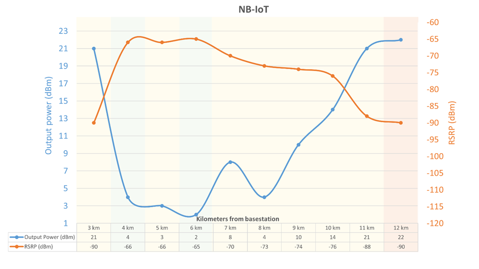
Figure 8 Correlation of Output power and RSRP on NB-IoT
Figure 8 shows the output power on the left axis and the RSRP on the right axis. The bottom table shows the kilometers from the base station (eNB) with the actual measurements. The background colors represent the energy estimates from Table 4, so we can see at 12 km it is estimated to be “poor conditions”.
Let us now look at how the power consumption in Figure 9 is affected by increasing the distance between the base station and the UE.
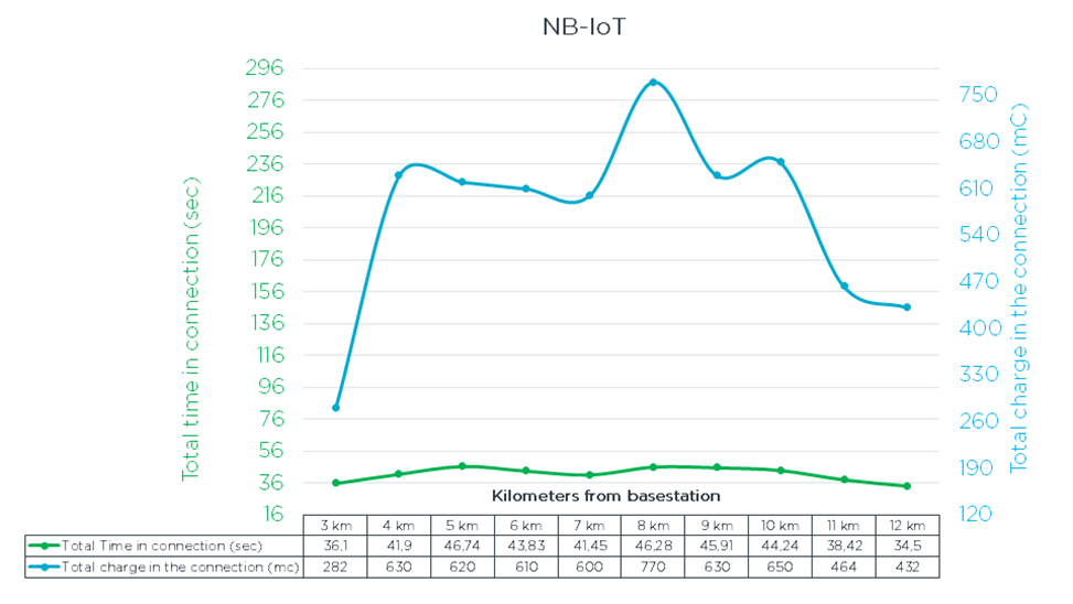
Figure 9 Total time and total charge captured during the connection in NB-IoT
From Figure 9, we can see the correlation between the total time in the connection and the total charge of the connection which is measured from the boot up of the nRF9160 SiP until it goes in Power Saving Mode. This can give you an overview of how the power consumption of a device is affected by distance (or obstructions) from the base station.
LTE-M and NB-IoT compared results
Let us bring together the data of Figure 6 andt Figure 8 into the same graph to compare output power and RSRP in Figure 10.
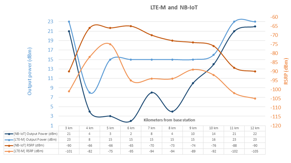
Figure 10 Correlation of Output power and RSRP on LTE-M and NB-IoT
From Figure 10 we see that NB-IoT has higher RSRP and lower output power than LTE-M from 3 km to 12 km. After that the LTE-M devices could not connect to the network, and the NB-IoT devices lost connection to the base station on Bitihorn. However, the NB-IoT devices actually got connected to another base station on a different location, so throughout the drive from 3 km to 17 km it was able to connect, but not for the original base station after 12 km.
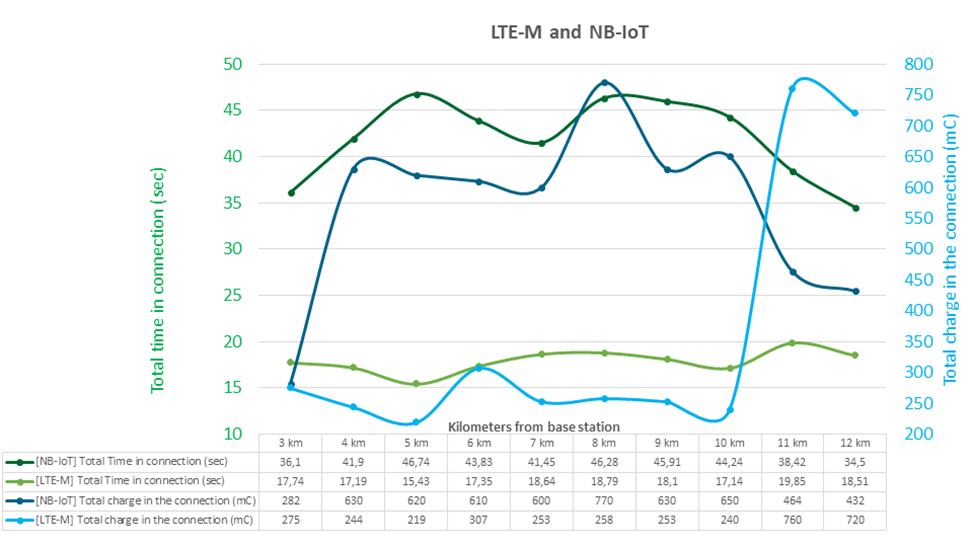
Figure 11 Total time and total charge captured during the connection in NB-IoT and LTE-M
In Figure 11, we are comparing the total time in connection and total charge in the connection for both LTE-M and NB-IoT.
Discussion
Network specific configurations
In Table 2, we see the different network-specific configurations assigned for the LTE-M and NB-IoT network that the UE cannot request to change. Notice that the RRC Inactivity timer is 7 seconds longer for NB-IoT compared to LTE-M. The longer timer is the network forcing the UE to stay in RRC Connected mode as a security measure since the network does not know when the last packet is sent, and results in more power the device will burn off. However, if the network supports it, this timer can be avoided by using the Release Assistant Indication (RAI) feature (%RAI AT command). RAI is used to indicate to the network that the last packet was sent, and that it can safely release the UE from RRC Connected Mode. This was not tested during this field test because of the current lack of support on the network side.
The other three network configuration values “cDRX interval”, “cDRX on duration” and “cDRX inactivity timer” will also impact the total power consumption, and we can show this by using the Online Power Profiler to estimate. Let us compare using the network configurations in Table 2 and disable RRC Idle mode, enable PSM and enable data transfers for 300 bytes in an interval of 1 hour. We will be using the same network mode “LTE-M” for simplicity while changing the network configurations to see the direct impact. Using the network configurations for the LTE-M section, the total average current equals 30.97µA while using the network configurations of NB-IoT results in a total average current of 18.3 µA. That is a decrease of 41% of the total average current just by having different network configurations! That is a big reason why you need to field test your network to check which network configurations you get in that area, because these configurations cannot be changed by the UE and will have a significant impact on the total power consumption. If they are bad, you need to push your network carrier on this and explain the impact this has on low power devices running on battery. These configurations can be arbitrary if the network does not know how much this can affect the battery life of constrained devices. This can potentially cut down years of your battery life depending on your application.
Just to clarify, recommended network configurations for low power devices are higher “cDRX interval” (up to a certain point), lower “cDRX on duration” and lower “cDRX inactivity timer.” All this is explained in detail in the GSMA white paper “Improving energy Efficiency for Mobile IoT”.
Distance and impact on signal strength for LTE-M and NB-IoT
Let us look at the difference of distance possible between the nRF9160 SiP (UE) and the base station (eNB) using LTE-M vs. NB-IoT. From Table 3 for LTE-M and Table 4 for NB-IoT we can see that we have a reliable connection between 3 km to 12 km using both the LTE-M technology and for the NB-IoT technology. The fact that LTE-M devices could not connect while the NB-IoT devices could connect, albeit other base stations, can be explained by the lower bandwidth of the NB-IoT technology, seen in Table 1.
The result at 3 km (closest to the eNB) for both LTE-M and NB-IoT (seen in Figure 6 and Figure 8 . This is explained by the small mountain obstructing seen in the red circle in Figure 12, where the blue circle is where our measurements were captured from. This is also clearly seen in Figure 13 (taken from Google maps) where the blue car icon is where we took the measurements, and the yellow circle is the eNB.
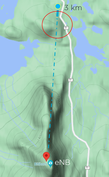
Figure 12 Measurements from 3 km away from the eNB
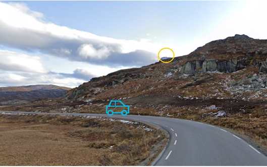
Figure 13 Measurement point (3 km) showing obstruction of the eNB
On the topic of distance, when we reached 11 to 12 km on the NB-IoT device, we can see from Figure 8 that the signal strength (RSRP) is reduced significantly, and the output power is increased to compensate. This affects the power consumption, first seen by the “Evaluating connection parameters” (%CONEVAL) feature responses in Table 4. We see that on 12 km the energy estimate is “poor conditions” for NB-IoT, which corresponds to “Setting up a connection might require retries and a higher number of repetitions for data” as stated in the documentation. Note that %CONEVAL is more beneficial to use in RRC Idle mode compared to how it is used in this field test (in RRC Connected) with regards to potentially saving power consumption.
Let us now look at how distance impacts the signal strength and output power on the nRF9160 DKs using the LTE-M technology. We see similar expected results in Figure 6 that the RSRP is high at the beginning and reduces as the distance increases from the eNB as well as the output power increases.
For both the LTE-M and NB-IoT devices we see a spike in RSRP decrease and output power increase at 11 km and 12 km in Figure 10. This could be explained by the fact that the data points are taken after a hill in the landscape, as seen in Figure 5.
Comparing LTE-M and NB-IoT on power consumption
First off, we need to consider both Table 1 Difference between LTE-M and NB-IoT and Table 2 Network specific configurations for LTE-M and NB-IoT on the eNB which is impacting the power consumption based on comparing these network configurations using the Online Power Profiler. The bandwidth of NB-IoT is lower which means the modem must stay longer in RRC Connected mode to accomplish the same amount of work. And we already discussed the impact of Network specific configurations in the beginning of the Discussion section.
Figure 11, displays a comparison of the total time in connection and total charge in the connection for both LTE-M and NB-IoT devices. We can see that the LTE-M device has an average of 61% shorter total time in connection compared to the NB-IoT device, which means a shorter amount of time using the radio which again should reflect in lower power consumption if they use the same network configurations. As we’ve seen, there are differences in the network configurations in this case (Table 2), but still not big enough to make an impact.
From the same figure we can see that in short distances (from 4 km up to 10 km) the LTE-M technology is using much less charge in the connection compared to the NB-IoT device, for the same amount of work. Only in worse conditions, at 3 km (because of the mountain obstruction, Figure 12) and 11 km and 12 km (because of the downhill behind the small top, Figure 5), did NB-IoT use less charge in the connection compared to LTE-M. This can, again, be explained by the lower bandwidth and the higher penetration properties of the NB-IoT technology. This shows that under normal conditions using LTE-M will on average have a lower power consumption than NB-IoT, but if you have devices deployed a long distance away from the eNB or with a lot of obstructions, then NB-IoT technology would be to prefer. Luckily when using nRF9160 SiP you can change the network technology at run time, which means you can optimize your application for different use cases where one technology would be more suited than the other. One fitting example for this is Firmware over the air (FOTA) updates, where it is highly recommended to use LTE-M because of the higher throughput. Also note that when the distance from the eNB increases, seen in Figure 9, to the device might have problems connecting to the network and can get stuck in network search for a long time. To prevent this, you can implement a safeguard in your application or utilize other features such as %MDMEV which will tell you early on that you will most likely not find a network and that you can quit the network search.
Limitations of the findings
A limitation is that we cannot compare the power measurement data and the data captured from the modem trace directly with full certainty since they were captured on two different devices. Therefore, it is a concern that the devices received different network parameters or used different amounts of time to search and connect to the network. In this analysis, we have assumed that the devices using the same network technology received similar network parameters and therefore got similar outcomes. This assumption is strengthened by the fact that we see similarities in the behavior and the trend impact of signal strength decreasing with power consumption measurements increasing.
Another limitations was that we did not receive the same exact network parameters from the NB-IoT network and the LTE-M network, but that also shows the reality and importance of field testing your device in a real network. Even if the networks are from the same base station and from the same carrier the network parameters may differ, and this is important to spot since it will have an impact on power consumption.
Conclusion
What we have seen in this field test is that when the distance from the eNB increases, the signal strength decreases and output power increases for both technologies. We also saw how obstructions and height differences in the landscape can influence the same parameters. We did also see the benefit of using the “Energy estimate” feature that gave us a rough estimate of the network conditions before sending any data. This is a beneficial tool for any low-power application so you can check the network environment before using it.
Another finding in this field test is the difference in power consumption between the two technologies. For normal conditions, LTE-M will use less power consumption, but when the device is in bad condition, up to a certain point, NB-IoT looks to possibly be the better option for sending lesser amounts of data. So there may be sweet spot where NB-IoT is more beneficial to use with regards to network conditions.
We also saw that NB-IoT has better range than LTE-M, since the NB-IoT devices connected to other base stations after 12 km although the RSRP and output power for those connections where quite low and high respectively. What we see from these results is that in most cases it is best to use LTE-M if you are focused on higher throughput and low power.
LTE abbreviations
- RSRP - reference signal received power.
- eNB - enhanced Node B. Base station/cell.
- RRC – Radio Resource Control
- PSM – Power Saving Mode
- cDRX – Connected Mode Discontinuous Reception
- iDRX – Idle Mode Discontinuous Reception
- eDRX – Extended Discontinuous Reception
- TX – Transmit
- RX - Receive
- UE - user equipment. Device connecting to base station. nRF9160 SiP in this field test.
- TAU – Tracking Area update
- UL - uplink. Packets from UE to eNB.
- DL - downlink. Packets from eNB to UE.
- Cell selection. UE procedure selecting which eNB to connect to.
- Cell reselection. UE procedure connects to another eNB.
- Cell handover. UE procedure to handover connection to another eNB.
Application files
Here are the application files used for this field test (Public_LTE-M_NB-IoT-fieldtest-samples.zip).

Top Comments